Code
!pip install dldna[colab] # in Colab
# !pip install dldna[all] # in your local

%load_ext autoreload
%autoreload 2 ![]()
“Simplicity is the ultimate sophistication.” - Leonardo da Vinci
Deep learning models have the powerful ability to express complex functions through numerous parameters. However, this ability can sometimes be a double-edged sword. When a model is overly fitted to the training data, the predictive performance on new data may actually decrease due to the overfitting phenomenon.
Since the resurgence of the backpropagation algorithm in 1986, overfitting has been a relentless challenge for deep learning researchers. Initially, they responded to overfitting by simply reducing the model size or increasing the training data. However, these methods were limited by their restriction on the model’s expressiveness or the difficulty of data collection. The emergence of AlexNet in 2012 opened a new era for deep learning but also highlighted the severity of the overfitting problem. AlexNet had many more parameters than previous models, increasing the risk of overfitting. As the scale of deep learning models increased exponentially thereafter, the overfitting problem became a core challenge in deep learning research.
In this chapter, we will explore the nature of overfitting and various techniques that have evolved to address it. Just as explorers navigate uncharted territories and create maps, deep learning researchers have continuously explored and developed new methods to overcome the obstacle of overfitting.
Overfitting was first mentioned in William Hopkins’ writings in 1670, but its modern meaning began with a mention in the Quarterly Review of Biology in 1935: “Analyzing six variables with 13 observations seems like overfitting.” It was formally studied in statistics starting in the 1950s, particularly in the context of time series analysis in the 1952 paper “Tests of Fit in Time Series.”
In deep learning, the overfitting problem entered a new phase with the emergence of AlexNet in 2012. AlexNet was a large-scale neural network with approximately 60 million parameters, unprecedented in scale compared to previous models. As the size of deep learning models increased exponentially thereafter, the overfitting problem became more severe. For example, modern large language models (LLMs) have billions of parameters, making overfitting prevention a core challenge in model design.
In response to these challenges, innovative solutions such as dropout (2014) and batch normalization (2015) were proposed. More recently, methods utilizing training history for overfitting detection and prevention (2024) are being researched. Especially in large models, various strategies are used in combination, from traditional methods like early stopping to modern techniques like ensemble learning and data augmentation.
Let’s intuitively understand the overfitting phenomenon through a simple example. We’ll apply polynomials of different degrees to noisy sine function data.
!pip install dldna[colab] # in Colab
# !pip install dldna[all] # in your local
%load_ext autoreload
%autoreload 2import numpy as np
import seaborn as sns
# Noisy sin graph
def real_func(x):
y = np.sin(x) + np.random.uniform(-0.2, 0.2, len(x))
return y
# Create x data from 40 to 320 degrees. Use a step value to avoid making it too dense.
x = np.array([np.pi/180 * i for i in range(40, 320, 4)])
y = real_func(x)
import seaborn as sns
sns.scatterplot(x=x, y=y, label='real function')
# Plot with 1st, 3rd, and 21th degree polynomials.
for deg in [1, 3, 21]:
# Get the coefficients for the corresponding degree using polyfit, and create the estimated function using poly1d.
params = np.polyfit(x, y, deg) # Get the parameter values
# print(f" {deg} params = {params}")
p = np.poly1d(params) # Get the line function
sns.lineplot(x=x, y=p(x), color=f"C{deg}", label=f"deg = {deg}")The autoreload extension is already loaded. To reload it, use:
%reload_ext autoreload/tmp/ipykernel_1362795/2136320363.py:25: RankWarning: Polyfit may be poorly conditioned
params = np.polyfit(x, y, deg) # Get the parameter values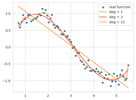
The code above generates noisy sine function data and fits it with 1st, 3rd, and 21st degree polynomials as an example.
1st degree function (deg = 1): The result is a simple line that does not follow the overall trend of the data. This shows a state of underfitting, where the model fails to capture the complexity of the data.
3rd degree function (deg = 3): It follows the basic pattern of the data relatively well, forming a smooth curve without being overly affected by noise.
21st degree function (deg = 21): The result shows overfitting, where the model follows the training data too closely, including its noise, and becomes overly optimized for only the training data.
Thus, if the complexity of the model (the degree of the polynomial in this case) is too low, underfitting occurs; if it’s too high, overfitting occurs. What we ultimately want to find is a model that generalizes well not just to the training data but also to new data - that is, an approximation function closest to the actual sine function.
Overfitting occurs when the complexity (or capacity) of the model is relatively high compared to the amount of training data. Neural networks are especially prone to overfitting because they have many parameters and high expressiveness. Overfitting can also occur when there’s not enough training data or when the data contains a lot of noise. The characteristics of overfitting include:
As a result, an overfitted model performs well on the training data but shows poor prediction performance on new, unseen data. To prevent such overfitting, we’ll explore various techniques like L1/L2 regularization, dropout, and batch normalization in more detail later.
Challenge: What methods can effectively control the complexity of a model while improving its generalization performance?
Researcher’s Dilemma: Reducing the size of a model to prevent overfitting may limit its expressiveness, and simply increasing the training data is not always possible. It was necessary to impose constraints on the model’s structure or learning process to prevent excessive optimization for the training data and improve predictive performance for new data.
In neural networks, L1 and L2 regularization are commonly used. L1 refers to Lasso regression, while L2 refers to Ridge regression.
Ridge regression and Lasso regression introduce a penalty term to restrict parameter movement. The differences between the two methods can be summarized in the following table:
| Feature | Ridge Regression | Lasso Regression |
|---|---|---|
| Penalty Type | Imposes an L2 penalty. The penalty term is the sum of the squares of the parameters multiplied by alpha. | Imposes an L1 penalty. The penalty term is the sum of the absolute values of the parameters multiplied by alpha. |
| Parameter Impact | Suppresses large parameters, making them close to 0, but not exactly 0 | Can set some parameter values to 0 when alpha is large, resulting in a simpler model |
| Overall Impact | Preserves all parameters, including those with minor effects | Selectively retains relevant parameters, allowing for a more straightforward explanation of complex models. |
| Optimization Characteristics | Less sensitive to ideal values compared to Lasso | Sensitive to ideal values due to the absolute value penalty term |
The equations can be expressed as follows:
Ridge Regression Objective Function
“Modified Ridge Objective Function” = (Unmodified Linear Regression Function) + \(\alpha \cdot \sum (\text{parameter})^2\)
\(f_{\beta} = \sum_{i=1}^{M} (y_i - \hat{y}_i)^2 + \alpha \sum_{j} \beta_{j}^2\)
Here, \(\beta\) is the parameter vector being sought. \(\alpha \sum_{j} \beta_{j}^2\) is the penalty term or regularization term. \(\alpha\) is a hyperparameter that controls the size of the regularization term. The formula for obtaining the parameters is as follows.
\(\beta = \underset{\beta}{\operatorname{argmin}} \left( \sum_{i=1}^{M} (y_i - \hat{y}_i)^2 + \alpha \sum_{j} \beta_{j}^2 \right)\)
Lasso Regression Objective Function
“Modified Lasso Objective Function” = (Unmodified Linear Regression Function) + $ || $
\(f_{\beta} = \sum_{i=1}^{M} (y_i - \hat{y}_i)^2 + \alpha \sum_{j} |\beta_{j}|\) \(\beta = \underset{\beta}{\operatorname{argmin}} \left( \sum_{i=1}^{M} (y_i - \hat{y}_i)^2 + \alpha \sum_{j} |\beta_j| \right)\) Using L2 with the sum of the squares of parameters as a penalty term is often referred to as weight decay in neural networks. Let’s take a look at how ridge (L2) regression differs from simple linear regression using sklearn’s implemented model. To do this, we need to increase the dimension of the input x data to the degree. We will use the following simple utility function to create it.
def get_x_powered(x, p=1):
    size = len(x)

    # The shape of the created x will be (data size, degree)
    new_x = np.zeros((size, p))

    for s in range(len(x)): # Iterate over data size
        for d in range(1, p+1): # Iterate over degrees
            new_x[s][d-1] = x[s]**d # Raise x to the power of the degree.

    return new_x


# Let's take a quick look at how it works.
deg = 3
x = np.array([np.pi/180 * i for i in range(20, 35, 5)])
y = real_func(x)  # real_func는 이전 코드에 정의되어 있다고 가정

print(f"x = {x}")
new_x = get_x_powered(x, p=deg)

print(f"new_x = {new_x}")
x = [0.34906585 0.43633231 0.52359878]
new_x = [[0.34906585 0.12184697 0.04253262]
[0.43633231 0.19038589 0.08307151]
[0.52359878 0.27415568 0.14354758]]Because it is third-order, the value of \(x\) increases to \(x^2, x^3\). For example, 0.3490, 0.1218 (the square of 0.3490), and 0.04253 (the cube of 0.3490) are examples. If it is tenth-order, data up to \(x^{10}\) is created. The alpha value of the penalty term can have a value from 0 to infinity. As the alpha value increases, the regulation intensity becomes larger. With the degree fixed at 13, we will compare the linear regression function and ridge regression by changing the alpha value.
import numpy as np
from sklearn.linear_model import Ridge
import matplotlib.pyplot as plt
import seaborn as sns
from sklearn.preprocessing import PolynomialFeatures
from sklearn.pipeline import make_pipeline

# Create a noisy sine wave (increased noise)
def real_func(x):
    return np.sin(x) + np.random.normal(0, 0.4, len(x))  # Increased noise

# Create x data (narrower range)
x = np.array([np.pi / 180 * i for i in range(40, 280, 8)])  # Narrower range, larger step

y = real_func(x)

# Degree of the polynomial
deg = 10

# List of alpha values to compare (adjusted)
alpha_list = [0.0, 0.1, 10]  # Adjusted alpha values
cols = len(alpha_list)

fig, axes_list = plt.subplots(1, cols, figsize=(20, 5))  # Adjusted figure size

for i, alpha in enumerate(alpha_list):
    axes = axes_list[i]

    # Plot the original data
    sns.scatterplot(ax=axes, x=x, y=y, label='real function', s=50)  # Increased marker size

    # Plot linear regression
    params = np.polyfit(x, y, deg)
    p = np.poly1d(params)
    sns.lineplot(ax=axes, x=x, y=p(x), label=f"LR deg = {deg}")

    # Ridge regression (using Pipeline, solver='auto')
    model = make_pipeline(PolynomialFeatures(degree=deg), Ridge(alpha=alpha, solver='auto'))
    model.fit(x.reshape(-1, 1), y)  # Reshape x for pipeline
    y_pred = model.predict(x.reshape(-1, 1)) # Reshape x for prediction
    sns.lineplot(ax=axes, x=x, y=y_pred, label=f"Ridge alpha={alpha:0.1e} deg={deg}")

    axes.set_title(f"Alpha = {alpha:0.1e}")
    axes.set_ylim(-1.5, 1.5)  # Limit y-axis range
    axes.legend()

plt.tight_layout()
plt.show()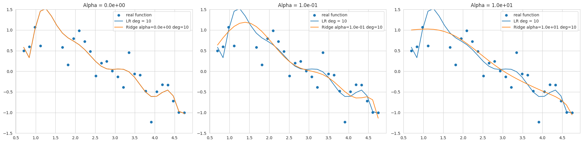
The above graph is the result of fitting a 10th degree polynomial to noisy sine function data, showing Ridge regression results with different alpha values (regularization strengths). The data range is narrow and noisy, so overfitting easily occurs even at low degrees.
alpha=0, but still sensitive to noise and far from the sine function.By selecting an appropriate alpha value, we can control model complexity and improve generalization performance. L2 regularization is useful for stabilizing models by making weights close to 0.
The sklearn.linear_model.Ridge model can have different optimization methods depending on the solver. Especially when the data range is narrow and noisy like this example, the 'svd' or 'cholesky' solver may be more stable, so careful selection of the solver is necessary (in the code, 'cholesky' is specified).
PyTorch and Keras have different ways of implementing L1 and L2 regularization. Keras supports adding regularization terms directly to each layer (kernel_regularizer, bias_regularizer).
# In Keras, you can specify regularization when declaring a layer.
keras.layers.Dense(64, activation='relu',
                    kernel_regularizer=regularizers.l2(0.01),
                    input_shape=(784,))
On the other hand, PyTorch applies L2 regularization by setting weight decay on the optimizer, and L1 regularization is typically implemented through a custom loss function.
import torch.nn as nn
import torch

def custom_loss(outputs, targets, model, lambda_l1=0.01, lambda_l2=0.01,):
    mse_loss = nn.MSELoss()(outputs, targets)

    l1_loss = 0.
    l2_loss = 0.
    for param in model.parameters():
        l1_loss += torch.sum(torch.abs(param)) # Take the absolute value of the parameters.
        l2_loss += torch.sum(param ** 2)  # Square the parameters.

    total_loss = mse_loss + lambda_l1 * l1_loss + lambda_l2 * l2_loss # Add L1 and L2 penalty terms to the loss.
    return total_loss

# Example usage within a training loop (not runnable as is)
# for inputs, targets in dataloader:
#     # ... (rest of the training loop)
#     loss = custom_loss(outputs, targets, model)
#     loss.backward()
    # ... (rest of the training loop)
As in the above example, you can define a custom_loss function to apply both L1 and L2 regularization. However, it is common to set the weight_decay corresponding to L2 regularization in the optimizer. But Adam and SGD optimizers implement weight decay slightly differently than L2 regularization. Traditional L2 regularization is to add a parameter squared term to the loss function.
\(L_{n+1} = L_{n} + \frac{ \lambda }{2} \sum w^2\)
Differentiating this with respect to the parameters gives:
\(\frac{\partial L_{n+1}}{\partial w} = \frac{\partial L_{n}}{\partial w} +\lambda w\)
SGD and Adam are implemented by directly adding the \(\lambda w\) term to the gradient. The SGD code in chapter_05/optimizers is as follows.
if self.weight_decay != 0:
    grad = grad.add(p, alpha=self.weight_decay)
This approach does not have exactly the same effect as adding an L2 regularization term to the loss function when combined with momentum or adaptive learning rate.
AdamW and Decoupled Weight Decay
The 2017 ICLR paper “Fixing Weight Decay Regularization in Adam” (https://arxiv.org/abs/1711.05101) pointed out that weight decay in the Adam optimizer works differently from L2 regularization, and proposed the AdamW optimizer to fix this issue. In AdamW, weight decay is decoupled from gradient updates and applied directly in the parameter update step. The code is in the same basic.py.
# PyTorch AdamW weght decay
if weight_decay != 0:
    param.data.mul_(1 - lr * weight_decay)
AdamW multiplies the parameter value by 1 - lr * weight_decay.
In conclusion, AdamW’s approach is closer to a more accurate implementation of L2 regularization. While it’s common to refer to SGD and Adam’s weight decay as L2 regularization due to historical reasons and similar effects, it’s more accurate to view them as separate regularization techniques, and AdamW clarifies this difference, providing better performance.
To visually understand the effect of L1 and L2 regularization on model learning, we will use the loss surface visualization technique introduced in Chapter 4. We compare the change in the loss surface with and without L2 regularization and observe how the location of the optimum changes with the strength of the regularization (weight_decay).
import sys

from dldna.chapter_05.visualization.loss_surface import xy_perturb_loss,  hessian_eigenvectors, visualize_loss_surface
from dldna.chapter_04.utils.data import get_dataset, get_device
from dldna.chapter_04.utils.metrics import load_model

import torch
import torch.nn as nn
import numpy as np
import torch.utils.data as data_utils
from torch.utils.data import  DataLoader


device = get_device()  # Get the device (CPU or CUDA)
train_dataset, test_dataset = get_dataset()  # Load the datasets.

act_name = "ReLU"
model_file = f"SimpleNetwork-{act_name}.pth"

small_dataset = data_utils.Subset(test_dataset, torch.arange(0, 256))  # Use a subset of the test dataset
data_loader = DataLoader(small_dataset, batch_size=256, shuffle=True)  # Create a data loader
loss_func = nn.CrossEntropyLoss()  # Define the loss function

# Load the trained model.
trained_model, _ = load_model(model_file=model_file, path="./tmp/opts/ReLU") # 4장의 load_model 사용
trained_model = trained_model.to(device)  # Move the model to the device

top_n = 2  # Number of top eigenvalues/eigenvectors to compute
top_eigenvalues, top_eigenvectors =  hessian_eigenvectors(model=trained_model, loss_func=loss_func, data_loader=data_loader, top_n=top_n, is_cuda=True)  # 5장의 함수 사용

d_min ,d_max, d_num = -1, 1, 50  # Define the range and number of points for the grid
lambda1, lambda2 = np.linspace(d_min, d_max, d_num).astype(np.float32), np.linspace(d_min, d_max, d_num).astype(np.float32)  # Create the grid of lambda values
x, y, z = xy_perturb_loss(model=trained_model, top_eigenvectors=top_eigenvectors, data_loader=data_loader, loss_func=loss_func, lambda1=lambda1, lambda2=lambda2, device=device) # 5장의 함수 사용
Create an approximate function with xy_perturb_loss, then put (x, y) into the approximate function again to obtain a new z value. The reason for doing this is that when drawing contours with the value obtained by xy_perturb_loss as in Chapter 5, the minimum value is slightly different, so the point of convergence of the optimizer deviates slightly. Now, without expressing all the paths the optimizer takes, only the last lowest point is compared while increasing the weight_decay value.
import torch
import numpy as np
import torch.nn as nn
import torch.optim as optim  # Import optim
import matplotlib.pyplot as plt
from torch.utils.data import DataLoader, Subset

# 5장, 4장 함수들 import
from dldna.chapter_05.visualization.loss_surface import (
    hessian_eigenvectors,
    xy_perturb_loss,
    visualize_loss_surface
)
from dldna.chapter_04.utils.data import get_dataset, get_device
from dldna.chapter_04.utils.metrics import load_model
from dldna.chapter_05.visualization.gaussian_loss_surface import (
    get_opt_params,
    train_loss_surface,
    gaussian_func # gaussian_func 추가.
)


device = get_device()
_, test_dataset = get_dataset(dataset="FashionMNIST")
small_dataset = Subset(test_dataset, torch.arange(0, 256))
data_loader = DataLoader(small_dataset, batch_size=256, shuffle=True)
loss_func = nn.CrossEntropyLoss()

act_name = "ReLU" # Tanh로 실험하려면 이 부분을 변경
model_file = f"SimpleNetwork-{act_name}.pth"
trained_model, _ = load_model(model_file=model_file, path="./tmp/opts/ReLU")
trained_model = trained_model.to(device)

top_n = 2
top_eigenvalues, top_eigenvectors = hessian_eigenvectors(
    model=trained_model,
    loss_func=loss_func,
    data_loader=data_loader,
    top_n=top_n,
    is_cuda=True
)

d_min, d_max, d_num = -1, 1, 30 # 5장의 30을 사용
lambda1 = np.linspace(d_min, d_max, d_num).astype(np.float32)
lambda2 = np.linspace(d_min, d_max, d_num).astype(np.float32)

x, y, z = xy_perturb_loss(
    model=trained_model,
    top_eigenvectors=top_eigenvectors,
    data_loader=data_loader,
    loss_func=loss_func,
    lambda1=lambda1,
    lambda2=lambda2,
    device=device # device 추가
)


# --- Optimization and Visualization ---

# Find the parameters that best fit the data.
popt, _, offset = get_opt_params(x, y, z)  # offset 사용

print(f"Optimal parameters: {popt}")

# Get a new z using the optimized surface function (Gaussian).
# No need for global g_offset, we can use the returned offset.
z_fitted = gaussian_func((x, y), *popt,offset) # offset을 더해야 함.


data = [(x, y, z_fitted)]  # Use z_fitted

axes = visualize_loss_surface(data, act_name=act_name, color="C0", size=6, levels=80, alpha=0.7, plot_3d=False)
ax = axes[0]

# Train with different weight decays and plot trajectories.
for n, weight_decay in enumerate([0.0, 6.0, 10.0, 18.0, 20.0]):
# for n, weight_decay in enumerate([0.0]):  # For faster testing
    points_sgd_m = train_loss_surface(
        lambda params: optim.SGD(params, lr=0.1, momentum=0.7, weight_decay=weight_decay),
        [d_min, d_max],
        200,
        (*popt, offset) # unpack popt and offset
    )
    ax.plot(
        points_sgd_m[-1, 0],
        points_sgd_m[-1, 1],
        color=f"C{n}",
        marker="o",
        markersize=10,
        zorder=2,
        label=f"wd={weight_decay:0.1f}"
    )
    ax.ticklabel_format(axis='both', style='scientific', scilimits=(0, 0))

plt.legend()
plt.show()
Function parameters = [ 4.59165436 0.34582255 -0.03204057 -1.09810435 1.54530407]
Optimal parameters: [ 4.59165436 0.34582255 -0.03204057 -1.09810435 1.54530407]
train_loss_surface: SGD
SGD: Iter=1 loss=4.7671 w=[-0.8065, 0.9251]
SGD: Iter=200 loss=1.9090 w=[0.3458, -0.0320]
train_loss_surface: SGD
SGD: Iter=1 loss=4.7671 w=[-0.2065, 0.3251]
SGD: Iter=200 loss=1.9952 w=[0.1327, -0.0077]
train_loss_surface: SGD
SGD: Iter=1 loss=4.7671 w=[0.1935, -0.0749]
SGD: Iter=200 loss=2.0293 w=[0.0935, -0.0051]
train_loss_surface: SGD
SGD: Iter=1 loss=4.7671 w=[0.9935, -0.8749]
SGD: Iter=200 loss=2.0641 w=[0.0587, -0.0030]
train_loss_surface: SGD
SGD: Iter=1 loss=4.7671 w=[1.1935, -1.0749]
SGD: Iter=200 loss=2.0694 w=[0.0537, -0.0027]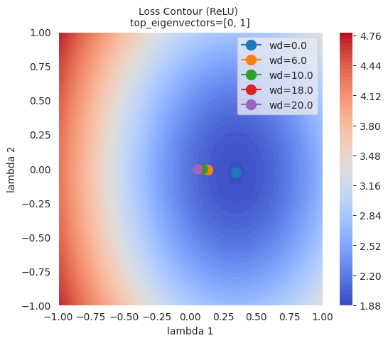
As can be seen in the figure, the larger the L2 regulation (weight decay), the farther the final point reached by the optimizer is from the lowest point of the loss function. This is because L2 regularization helps prevent the model from overfitting by preventing the weights from becoming too large.
L1 regularization creates a sparse model by making some weights 0. It is useful when you want to reduce the complexity of the model and remove unnecessary features. On the other hand, L2 regularization does not make the weights completely 0, but keeps all weights small. L2 regularization is generally more stable and is also called ‘soft regularization’ because it gradually reduces the weights.
L1 and L2 regularizations are applied differently depending on the characteristics of the problem, data, and purpose of the model. While L2 regularization is generally more widely used, it is a good idea to try both and see which one performs better in some cases. Additionally, Elastic Net regularization, which combines L1 and L2 regularization, can also be considered.
Elastic Net is a regularization method that combines L1 and L2 regulations. By taking the advantages of each regulation and compensating for their disadvantages, it can create more flexible and effective models.
Key Points:
Formula:
The cost function of Elastic Net is expressed as follows:
\(Cost = Loss + \lambda_1 \sum_{i} |w_i| + \lambda_2 \sum_{i} (w_i)^2\)
Loss: The original model’s loss function (e.g., MSE, Cross-Entropy)λ₁: A hyperparameter that controls the strength of L1 regulationλ₂: A hyperparameter that controls the strength of L2 regulationwᵢ: The model’s weightsAdvantages:
λ₁ and λ₂. If λ₁=0, it becomes L2 regulation (Ridge), and if λ₂=0, it becomes L1 regulation (Lasso).Disadvantages:
λ₁ and λ₂, which can be more complex than tuning L1 or L2 regulation.Applicable Cases:
Summary: Elastic Net is a powerful regularization method that combines the advantages of L1 and L2 regulations. Although hyperparameter tuning is required, it can perform well in various problems.
Dropout is one of the powerful regularization methods to prevent overfitting in neural networks. During the training process, some neurons are randomly deactivated (dropped out) to prevent specific neurons or combinations of neurons from becoming too dependent on the training data. This has a similar effect to ensemble learning, where multiple people learn different parts and then combine their strengths to solve a problem. Each neuron is encouraged to learn important features independently, improving the model’s generalization performance. It is typically applied to fully connected layers, with a dropout rate of 20% to 50%. Dropout is only applied during training, and all neurons are used during inference.
Dropout can be implemented in PyTorch as follows.
import torch.nn as nn

class Dropout(nn.Module):
    def __init__(self, dropout_rate):
        super(Dropout, self).__init__()
        self.dropout_rate = dropout_rate

    def forward(self, x):
        if self.training:
            mask = torch.bernoulli(torch.ones_like(x) * (1 - self.dropout_rate)) / (1 - self.dropout_rate)
            return x * mask
        else:
            return x

# Usage example.  Drops out 0.5 (50%).
dropout = Dropout(dropout_rate=0.5)

# Example input data
inputs = torch.randn(1000, 100)

# Forward pass (during training)
dropout.train()
outputs_train = dropout(inputs)

# Forward pass (during inference)
dropout.eval()
outputs_test = dropout(inputs)

print("Input shape:", inputs.shape)
print("Training output shape:", outputs_train.shape)
print("Test output shape", outputs_test.shape)
print("Dropout rate (should be close to 0.5):", 1 - torch.count_nonzero(outputs_train) / outputs_train.numel())
Input shape: torch.Size([1000, 100])
Training output shape: torch.Size([1000, 100])
Test output shape torch.Size([1000, 100])
Dropout rate (should be close to 0.5): tensor(0.4997)The implementation is very simple. It multiplies the mask value to the input tensor and inactivates a certain percentage of neurons. The dropout layer does not have separate learnable parameters, but simply plays the role of randomly making some of the inputs 0. In actual neural networks, the dropout layer is used by inserting it between other layers (e.g., linear layers, convolutional layers).
Dropout removes neurons randomly during training, but uses all neurons during inference. To match the scale of output values between training and inference, the inverted dropout method is used. Inverted dropout performs scaling in advance by dividing by (1 - dropout_rate) during training, so that it can be used as is without additional calculations during inference. This allows achieving an effect similar to ensemble learning during inference, i.e., averaging multiple sub-networks, while also improving computational efficiency.
Let’s take a look at how effective dropout is through a graph using simple data. The source code is chapter_06/plot_dropout.py, and we will omit introducing the unimportant code due to space constraints. Since it has detailed comments, it’s not difficult to look at the source code. When drawing the graph, we can see that the model with dropout applied (blue) has a much higher test accuracy.
from dldna.chapter_06.plot_dropout import plot_dropout_effect

plot_dropout_effect()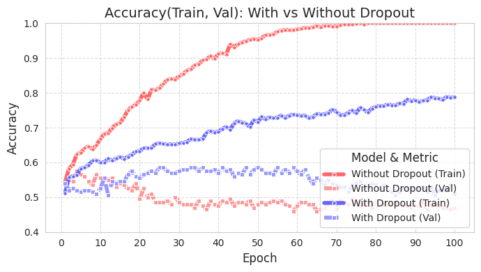
The training accuracy of the model with dropout (With Dropout) is lower than that of the model without dropout (Without Dropout), but the validation accuracy is higher. This means that dropout reduces overfitting to the training data and improves the generalization performance of the model.
Batch normalization plays a role in regularization and also increases the stability of data during training. Batch normalization was first proposed in the 2015 paper by Ioffe and Szegedy [Reference 2]. In deep learning, as data passes through each layer, the distribution of activation values changes, causing an internal covariate shift. This slows down the training speed and makes the model unstable (since the distribution changes, more calculation steps are required). This problem becomes more severe as the number of layers increases. Batch normalization mitigates this by normalizing the data in mini-batch units.
The core idea of batch normalization is to normalize the data in mini-batch units. The following code illustrates this easily.
# Calculate the mean and variance of the mini-batch
batch_mean = x.mean(dim=0)
batch_var = x.var(dim=0, unbiased=False)

# Perform normalization
x_norm = (x - batch_mean) / torch.sqrt(batch_var + epsilon)

# Apply scale and shift parameters
y = gamma * x_norm + beta
Generally, batch normalization uses the variance and mean of the data within a single mini-batch to normalize the entire data, bringing about distributional changes. It first performs normalization, then applies a certain scale parameter and shift parameter. The gamma above is the scale parameter, and beta is the shift parameter. It’s helpful to think of it simply as \(y = ax + b\). The epsilon used during normalization is a very small constant value (1e-5 or 1e-7) that often appears in numerical analysis, and is used for numerical stability. Batch normalization provides the following additional effects:
Let’s compare the case where pure normalization is applied to randomly generated data with two features, and the case where scale and shift parameters are applied, using a graph. Through visualization, we can easily understand the numerical meaning of normalization for mini-batches.
import numpy as np
import seaborn as sns
import matplotlib.pyplot as plt

# Generate data
np.random.seed(42)
x = np.random.rand(50, 2) * 10

# Batch normalization (including scaling parameters)
def batch_normalize(x, epsilon=1e-5, gamma=1.0, beta=0.0):
    mean = x.mean(axis=0)
    var = x.var(axis=0)
    x_norm = (x - mean) / np.sqrt(var + epsilon)
    x_scaled = gamma * x_norm + beta
    return x_norm, mean, x_scaled

# Perform normalization (gamma=1.0, beta=0.0 is pure normalization)
x_norm, mean, x_norm_scaled = batch_normalize(x, gamma=1.0, beta=0.0)
# Perform normalization and scaling (apply gamma=2.0, beta=1.0)
_, _, x_scaled = batch_normalize(x, gamma=2.0, beta=1.0)

# Set Seaborn style
sns.set_style("whitegrid")
sns.set_context("notebook", font_scale=1.2)

# Visualization
fig, (ax1, ax2, ax3) = plt.subplots(1, 3, figsize=(18, 5))

# Original data
sns.scatterplot(x=x[:, 0], y=x[:, 1], ax=ax1, color='royalblue', alpha=0.7)
ax1.scatter(mean[0], mean[1], color='red', marker='*', s=200, label='Mean')
ax1.set(title='Original Data',
        xlabel='Feature 1',
        ylabel='Feature 2',
        xlim=(-2, 12),
        ylim=(-2, 12))
ax1.legend()

# After normalization (gamma=1, beta=0)
sns.scatterplot(x=x_norm[:, 0], y=x_norm[:, 1], ax=ax2, color='crimson', alpha=0.7)
ax2.scatter(0, 0, color='blue', marker='*', s=200, label='Mean (0,0)')
ax2.axhline(y=0, color='k', linestyle='--', alpha=0.3)
ax2.axvline(x=0, color='k', linestyle='--', alpha=0.3)
ax2.set(title='After Normalization (γ=1, β=0)',
        xlabel='Normalized Feature 1',
        ylabel='Normalized Feature 2',
        xlim=(-2, 12),
        ylim=(-2, 12))
ax2.legend()

# After scaling and shifting (gamma=2, beta=1)
sns.scatterplot(x=x_scaled[:, 0], y=x_scaled[:, 1], ax=ax3, color='green', alpha=0.7)
ax3.scatter(1, 1, color='purple', marker='*', s=200, label='New Mean')
ax3.axhline(y=1, color='k', linestyle='--', alpha=0.3)
ax3.axvline(x=1, color='k', linestyle='--', alpha=0.3)
ax3.set(title='After Scale & Shift (γ=2, β=1)',
        xlabel='Scaled Feature 1',
        ylabel='Scaled Feature 2',
        xlim=(-2, 12),
        ylim=(-2, 12))
ax3.legend()

plt.tight_layout()
plt.show()

# Print statistics
print("\nOriginal Data Statistics:")
print(f"Mean: {mean}")
print(f"Variance: {x.var(axis=0)}")

print("\nNormalized Data Statistics (γ=1, β=0):")
print(f"Mean: {x_norm.mean(axis=0)}")
print(f"Variance: {x_norm.var(axis=0)}")

print("\nScaled Data Statistics (γ=2, β=1):")
print(f"Mean: {x_scaled.mean(axis=0)}")
print(f"Variance: {x_scaled.var(axis=0)}")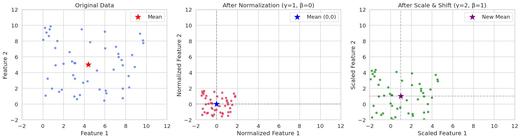
Original Data Statistics:
Mean: [4.40716778 4.99644709]
Variance: [8.89458134 8.45478364]

Normalized Data Statistics (γ=1, β=0):
Mean: [-2.70894418e-16 -3.59712260e-16]
Variance: [0.99999888 0.99999882]

Scaled Data Statistics (γ=2, β=1):
Mean: [1. 1.]
Variance: [3.9999955  3.99999527]
In seed(42), you can often see that the random initial value is set to 42. This is a programmer’s habit, and other numbers can also be used. 42 is a number that appears in Douglas Adams’ novel “The Hitchhiker’s Guide to the Galaxy” as the “answer to life, the universe, and everything”. Therefore, it is often used as an example code among programmers.
In PyTorch, the implementation typically involves inserting batch normalization layers into neural network layers. The following is an example.
import torch.nn as nn

class SimpleNet(nn.Module):
    def __init__(self):
        super().__init__()
        self.network = nn.Sequential(
            nn.Linear(784, 256),
            nn.BatchNorm1d(256),  # 배치 정규화 층
            nn.ReLU(),
            nn.Linear(256, 10)
        )

    def forward(self, x):
        return self.network(x)
PyTorch batch normalization implementation based on the original source code can be simplified as follows, and as done in the previous chapter, it is implemented briefly for learning purposes.
import torch
import torch.nn as nn

class BatchNorm1d(nn.Module):
    def __init__(self, num_features, eps=1e-5, momentum=0.1):
        super().__init__()
        self.num_features = num_features
        self.eps = eps
        self.momentum = momentum

        # Trainable parameters
        self.gamma = nn.Parameter(torch.ones(num_features))  # scale
        self.beta = nn.Parameter(torch.zeros(num_features))  # shift

        # Running statistics to be tracked
        self.register_buffer('running_mean', torch.zeros(num_features))
        self.register_buffer('running_var', torch.ones(num_features))

    def forward(self, x):
        if self.training:
            # Calculate mini-batch statistics
            batch_mean = x.mean(dim=0)  # Mean per channel
            batch_var = x.var(dim=0, unbiased=False)  # Variance per channel

            # Update running statistics (important)
            self.running_mean = (1 - self.momentum) * self.running_mean + self.momentum * batch_mean
            self.running_var = (1 - self.momentum) * self.running_var + self.momentum * batch_var

            # Normalize
            x_norm = (x - batch_mean) / torch.sqrt(batch_var + self.eps)

        else:
            # During inference, use the stored statistics
            x_norm = (x - self.running_mean) / torch.sqrt(self.running_var + self.eps)

        # Apply scale and shift
        return self.gamma * x_norm + self.beta
The biggest difference from the basic implementation is the part that updates statistics during execution. During training, it allows you to finally know the overall average and variance by accumulating the statistical values (average and variance) of the mini-batch as it moves. To track the movement, an exponential moving average (Exponential Moving Average) using momentum (default 0.1) is used. By using the average and variance obtained during training for inference, accurate variance and deviation are applied to the inference data, ensuring consistency between learning and inference.
Of course, this implementation is highly simplified for learning purposes. The location of the reference code is (https://github.com/pytorch/pytorch/blob/main/torch/nn/modules/batchnorm.py). The actual implementation of BatchNorm1d is much more complex. This is because frameworks such as PyTorch and TensorFlow typically include various logic beyond basic logic, including CUDA optimization, gradient optimization, handling various settings, and linking with C/C++.
Batch normalization (BN), proposed by Ioffe & Szegedy in 2015, has become a key technique in deep learning model training. BN accelerates the learning speed by normalizing the input of each layer, alleviates the vanishing/exploding gradient problem, and provides some regularization effect. In this deep dive, we will examine the forward and backward pass processes of BN in detail and analyze its effects mathematically.
Batch normalization is performed on a mini-batch basis. Given a mini-batch size of \(B\) and a feature dimension of \(D\), the mini-batch input data can be represented as a \(B \times D\) matrix \(\mathbf{X}\). Since BN operates independently for each feature dimension, we will consider only one feature dimension for explanation.
Mini-Batch Mean Calculation:
\(\mu_B = \frac{1}{B} \sum_{i=1}^{B} x_i\)
Here, \(x_i\) represents the value of the corresponding feature for the \(i\)th sample in the mini-batch.
Mini-Batch Variance Calculation:
\(\sigma_B^2 = \frac{1}{B} \sum_{i=1}^{B} (x_i - \mu_B)^2\)
Normalization:
\(\hat{x_i} = \frac{x_i - \mu_B}{\sqrt{\sigma_B^2 + \epsilon}}\)
Here, \(\epsilon\) is a small constant to prevent the denominator from being zero.
Scaling and Shifting:
\(y_i = \gamma \hat{x_i} + \beta\)
Here, \(\gamma\) and \(\beta\) are learnable parameters responsible for scaling and shifting, respectively. These parameters restore the representation power of the normalized data.
The backward pass of batch normalization involves calculating the gradients of the loss function with respect to each parameter using the chain rule. The process can be visually represented through a computational graph as follows (simplified using ASCII art):
     x_i   -->   [-]   -->   [/]   -->   [*]   -->   [+]   -->   y_i
      |          ^          ^          ^          ^
      |          |          |          |          |
      |          |          |          |          +---> beta
      |          |          |          +---> gamma
      |          |          +---> sqrt(...) + epsilon
| +---> mu_B, sigma_B^2Calculation of \(\frac{\partial \mathcal{L}}{\partial \beta}\) and \(\frac{\partial \mathcal{L}}{\partial \gamma}\):
\(\frac{\partial \mathcal{L}}{\partial \beta} = \sum_{i=1}^{B} \frac{\partial \mathcal{L}}{\partial y_i} \cdot \frac{\partial y_i}{\partial \beta} = \sum_{i=1}^{B} \frac{\partial \mathcal{L}}{\partial y_i}\)
\(\frac{\partial \mathcal{L}}{\partial \gamma} = \sum_{i=1}^{B} \frac{\partial \mathcal{L}}{\partial y_i} \cdot \frac{\partial y_i}{\partial \gamma} = \sum_{i=1}^{B} \frac{\partial \mathcal{L}}{\partial y_i} \cdot \hat{x_i}\)
Calculation of \(\frac{\partial \mathcal{L}}{\partial \hat{x_i}}\):
\(\frac{\partial \mathcal{L}}{\partial \hat{x_i}} = \frac{\partial \mathcal{L}}{\partial y_i} \cdot \frac{\partial y_i}{\partial \hat{x_i}} = \frac{\partial \mathcal{L}}{\partial y_i} \cdot \gamma\)
Calculation of \(\frac{\partial \mathcal{L}}{\partial \sigma_B^2}\):
\(\frac{\partial \mathcal{L}}{\partial \sigma_B^2} = \sum_{i=1}^{B} \frac{\partial \mathcal{L}}{\partial \hat{x_i}} \cdot \frac{\partial \hat{x_i}}{\partial \sigma_B^2} = \sum_{i=1}^{B} \frac{\partial \mathcal{L}}{\partial \hat{x_i}} \cdot (x_i - \mu_B) \cdot (-\frac{1}{2})(\sigma_B^2 + \epsilon)^{-3/2}\)
Calculation of \(\frac{\partial \mathcal{L}}{\partial \mu_B}\):
\(\frac{\partial \mathcal{L}}{\partial \mu_B} = \sum_{i=1}^{B} \frac{\partial \mathcal{L}}{\partial \hat{x_i}} \cdot \frac{\partial \hat{x_i}}{\partial \mu_B} + \frac{\partial \mathcal{L}}{\partial \sigma_B^2} \cdot \frac{\partial \sigma_B^2}{\partial \mu_B} = \sum_{i=1}^{B} \frac{\partial \mathcal{L}}{\partial \hat{x_i}} \cdot \frac{-1}{\sqrt{\sigma_B^2 + \epsilon}} + \frac{\partial \mathcal{L}}{\partial \sigma_B^2} \cdot (-2)\frac{1}{B}\sum_{i=1}^B (x_i-\mu_B)\)
Since \(\sum_{i=1}^B (x_i - \mu_B) = 0\) \(\frac{\partial \mathcal{L}}{\partial \mu_B} = \sum_{i=1}^{B} \frac{\partial \mathcal{L}}{\partial \hat{x_i}} \cdot \frac{-1}{\sqrt{\sigma_B^2 + \epsilon}}\)
\(\frac{\partial \mathcal{L}}{\partial x_i}\) calculation:
\(\frac{\partial \mathcal{L}}{\partial x_i} = \frac{\partial \mathcal{L}}{\partial \hat{x_i}} \cdot \frac{\partial \hat{x_i}}{\partial x_i} + \frac{\partial \mathcal{L}}{\partial \mu_B} \cdot \frac{\partial \mu_B}{\partial x_i} + \frac{\partial \mathcal{L}}{\partial \sigma_B^2} \cdot \frac{\partial \sigma_B^2}{\partial x_i} = \frac{\partial \mathcal{L}}{\partial \hat{x_i}} \cdot \frac{1}{\sqrt{\sigma_B^2 + \epsilon}} + \frac{\partial \mathcal{L}}{\partial \mu_B} \cdot \frac{1}{B} + \frac{\partial \mathcal{L}}{\partial \sigma_B^2} \cdot \frac{2}{B}(x_i - \mu_B)\)
Batch normalization prevents the input of each layer from becoming extremely large or small by normalizing it, which helps alleviate the gradient vanishing/exploding problems that occur in activation functions such as sigmoid or tanh.
During training, batch normalization calculates the mean and variance for each mini-batch, but during inference, it requires an estimate of the mean and variance of the entire training data. To achieve this, batch normalization calculates the running mean and running variance during training.
Running Mean Calculation:
\(\text{running\_mean} = (1 - \text{momentum}) \times \text{running\_mean} + \text{momentum} \times \mu_B\)
Running Variance Calculation:
\(\text{running\_var} = (1 - \text{momentum}) \times \text{running\_var} + \text{momentum} \times \sigma_B^2\)
Here, momentum is a hyperparameter that is typically set to a small value such as 0.1 or 0.01.
During inference, the running_mean and running_var calculated during training are used to normalize the input.
Batch Normalization (BN): uses statistics from within the mini-batch of samples. It is affected by batch size and is difficult to apply to RNNs.
Layer Normalization (LN): uses statistics from within each sample over the feature dimension. It is not affected by batch size and is easy to apply to RNNs.
Instance Normalization (IN): calculates statistics independently for each sample and each channel. It is mainly used in image generation tasks such as style transfer.
Group Normalization (GN): divides channels into groups and calculates statistics within each group. It can be used as an alternative to BN when the batch size is small.
Each normalization technique has its own strengths and weaknesses under different circumstances, so it’s necessary to choose the right technique according to the characteristics of the problem and model architecture.
Hyperparameter optimization has a significant impact on model performance. Its importance began to be recognized in the 1990s. In the late 1990s, it was discovered in Support Vector Machines (SVM) that even with the same model, the parameters of the kernel function (C, gamma, etc.) played a crucial role in performance. Around 2015, it was proven that Bayesian optimization yields better results than manual tuning, which became the core foundation for automated tuning methods like Google AutoML (2017).
There are several methods to optimize hyperparameters. The representative methods are as follows:
Grid Search: The most basic method, where possible values for each hyperparameter are listed and all combinations of these values are tried. It is useful when the number of hyperparameters is small and the range of values each parameter can take is limited, but it incurs high computational costs because all combinations must be tested. It is suitable for testing simple models or when the search space is very small.
Random Search: Hyperparameter values are randomly selected to create combinations, and these combinations are used to train the model and evaluate its performance. If some hyperparameters have a significant impact on performance, it can be more effective than grid search (Bergstra & Bengio, 2012).
Bayesian Optimization: Based on previous search results, a probabilistic model (usually Gaussian process) is used to intelligently select the next hyperparameter combination to try. It selects the next exploration point by maximizing an acquisition function. By efficiently exploring the hyperparameter search space, it can find better combinations with fewer trials than grid search or random search.
There are also other methods such as evolutionary algorithms using genetic algorithms and gradient-based optimization.
The following is an example of optimizing hyperparameters for a simple neural network model using Bayesian optimization.
Bayesian optimization began to gain attention in the 2010s. Especially after the publication of the paper “Practical Bayesian Optimization of Machine Learning Algorithms” in 2012, it has become one of the main methods for optimizing hyperparameters of deep learning models. Unlike grid search or random search, its significant advantage is that it intelligently selects the next parameter to explore based on previous trial results.
Bayesian optimization largely repeats the following three steps:
init_points.import torch
import torch.nn as nn
import torch.optim as optim
from dldna.chapter_04.models.base import SimpleNetwork
from dldna.chapter_04.utils.data import get_data_loaders, get_device
from bayes_opt import BayesianOptimization
from dldna.chapter_04.experiments.model_training import train_model, eval_loop
def train_simple_net(hidden_layers, learning_rate, batch_size, epochs):
"""Trains a SimpleNetwork model with given hyperparameters.
Uses CIFAR100 dataset and train_model from Chapter 4.
"""
device = get_device() # Use the utility function to get device
# Get data loaders for CIFAR100
train_loader, test_loader = get_data_loaders(dataset="CIFAR100", batch_size=batch_size)
# Instantiate the model with specified activation and hidden layers.
# CIFAR100 images are 3x32x32, so the input size is 3*32*32 = 3072.
model = SimpleNetwork(act_func=nn.ReLU(), input_shape=3*32*32, hidden_shape=hidden_layers, num_labels=100).to(device)
# Optimizer: Use Adam
optimizer = optim.Adam(model.parameters(), lr=learning_rate)
# Train the model using the training function from Chapter 4
results = train_model(model, train_loader, test_loader, device, optimizer=optimizer, epochs=epochs, save_dir="./tmp/tune",
retrain=True) # retrain=True로 설정
# Return the final test accuracy
return results['test_accuracies'][-1]
def train_wrapper(learning_rate, batch_size, hidden1, hidden2):
"""Wrapper function for Bayesian optimization."""
return train_simple_net(
hidden_layers=[int(hidden1), int(hidden2)],
learning_rate=learning_rate,
batch_size=int(batch_size),
epochs=10
)
def optimize_hyperparameters():
"""Runs hyperparameter optimization."""
# Set the parameter ranges to be optimized.
pbounds = {
"learning_rate": (1e-4, 1e-2),
"batch_size": (64, 256),
"hidden1": (64, 512), # First hidden layer
"hidden2": (32, 256) # Second hidden layer
}
# Create a Bayesian optimization object.
optimizer = BayesianOptimization(
f=train_wrapper,
pbounds=pbounds,
random_state=1,
allow_duplicate_points=True
)
# Run optimization
optimizer.maximize(
init_points=4,
n_iter=10,
)
# Print the best parameters and accuracy
print("\nBest parameters found:")
print(f"Learning Rate: {optimizer.max['params']['learning_rate']:.6f}")
print(f"Batch Size: {int(optimizer.max['params']['batch_size'])}")
print(f"Hidden Layer 1: {int(optimizer.max['params']['hidden1'])}")
print(f"Hidden Layer 2: {int(optimizer.max['params']['hidden2'])}")
print(f"\nBest accuracy: {optimizer.max['target']:.4f}")
if __name__ == "__main__":
print("Starting hyperparameter optimization...")
optimize_hyperparameters()The above example performs hyperparameter optimization using the BayesOpt package. The SimpleNetwork (defined in Chapter 4) is used as the training target, and the CIFAR100 dataset is used. The train_wrapper function serves as the objective function for BayesOpt, training the model with a given combination of hyperparameters and returning the final test accuracy.
pbounds specifies the search range for each hyperparameter. In optimizer.maximize, init_points is the number of initial random searches, and n_iter is the number of Bayesian optimization iterations. Therefore, the total number of experiments is init_points + n_iter.
When searching for hyperparameters, note the following:
n_iter.The BoTorch framework has recently gained attention in the field of deep learning hyperparameter optimization. BoTorch is a Bayesian optimization framework based on PyTorch, developed by FAIR (Facebook AI Research, now Meta AI) in 2019. Bayes-Opt is an older Bayesian optimization library that has been developed since 2016 and provides an intuitive and simple interface (scikit-learn style API), making it widely used.
The advantages and disadvantages of the two libraries are clear.
Therefore, Bayes-Opt is suitable for simple problems or rapid prototyping, while BoTorch is recommended for complex hyperparameter optimization of deep learning models, large-scale/high-dimensional problems, or advanced Bayesian optimization techniques (e.g., multi-task, constrained optimization).
To use BoTorch, unlike Bayes-Opt, you need to understand a few key concepts required for initial setup: surrogate models, input data normalization, and acquisition functions.
Surrogate Model:
A surrogate model is a model that approximates the actual objective function (in this case, the validation accuracy of a deep learning model). Typically, a Gaussian process (GP) is used. GP is used to predict results quickly and cheaply instead of the actual objective function, which can be computationally expensive. BoTorch provides the following GP models:
SingleTaskGP: The most basic Gaussian process model, suitable for single-objective optimization problems and effective with relatively small datasets (less than 1000 data points).MultiTaskGP: Used for multi-objective optimization problems where multiple objective functions are optimized simultaneously. For example, you can optimize both the accuracy and inference time of a model.SAASBO (Sparsity-Aware Adaptive Subspace Bayesian Optimization): A model specialized for high-dimensional parameter spaces. It assumes sparsity in high-dimensional spaces and performs efficient exploration.Input Data Normalization:
Gaussian processes are sensitive to the scale of the data, so normalizing the input data (hyperparameters) is crucial. Typically, all hyperparameters are transformed to the range [0, 1]. BoTorch provides Normalize and Standardize transformations.
Acquisition Function:
The acquisition function determines the next point to evaluate based on the current surrogate model. It balances exploration (searching for new areas) and exploitation (focusing on areas with high predicted performance). Common acquisition functions include probability of improvement (PI), expected improvement (EI), and Thompson sampling. BoTorch provides a variety of acquisition functions, including ProbabilityOfImprovement, ExpectedImprovement, and UpperConfidenceBound. The acquisition function is based on a surrogate model (GP) and is used to determine the next hyperparameter combination to experiment with. The acquisition function balances the trade-off between “exploration” and “exploitation”. BoTorch provides the following various acquisition functions.
ExpectedImprovement (EI): One of the most common acquisition functions, considering both the probability of getting a better result than the current optimum and the magnitude of improvement.LogExpectedImprovement (LogEI): A log-transformed version of EI, which is numerically more stable and sensitive to small changes.UpperConfidenceBound (UCB): An acquisition function that focuses more on exploration, actively exploring areas with high uncertainty.ProbabilityOfImprovement (PI): Represents the probability of improvement over the current optimum.qExpectedImprovement (qEI): Also known as q-batch EI, used for parallel optimization, selecting multiple candidates at once.qNoisyExpectedImprovement (qNEI): Q-batch Noisy EI, used in noisy environments.The entire code is located in package/botorch_optimization.py and can be run directly from the command line. Since the full code contains detailed comments, we will only explain the important parts here.
def __init__(self, max_trials: int = 80, init_samples: int = 10):
    self.param_bounds = torch.tensor([
        [1e-4, 64.0, 32.0, 32.0],      # 최소값
        [1e-2, 256.0, 512.0, 512.0]    # 최대값
    ], dtype=torch.float64)
In the initialization part, the minimum and maximum values of each hyperparameter are set. max_trials is the total number of attempts, and init_samples is the initial number of random experiments (same as init_points in Bayes-Opt). init_samples is typically set to 2-3 times the number of parameters. In the above example, since there are 4 hyperparameters, around 8-12 would be suitable. torch.float64 is used for numerical stability. Bayesian optimization, especially Gaussian process, uses Cholesky decomposition when calculating kernel matrices, and in this process, float32 can cause errors due to precision issues.
def tune(self):
    # 가우시안 프로세스 모델 학습
    model = SingleTaskGP(configs, accuracies)
    mll = ExactMarginalLogLikelihood(model.likelihood, model)
    fit_gpytorch_mll(mll)
We use SingleTaskGP as a surrogate model based on Gaussian processes. ExactMarginalLogLikelihood is the loss function for model training, and fit_gpytorch_mll trains the model using this loss function.
acq_func = LogExpectedImprovement(
    model,
    best_f=accuracies.max().item()
)
The acquisition function used is LogExpectedImprovement. It uses a log, so it has high numerical stability and is sensitive to small changes.
candidate, _ = optimize_acqf(                                   # 획득 함수 최적화로 다음 실험할 파라미터 선택
    acq_func, bounds=bounds,                                    # 획득 함수와 파라미터 범위 지정
    q=1,                                                        # 한 번에 하나의 설정만 선택
    num_restarts=10,                                            # 최적화 재시작 횟수
    raw_samples=512                                             # 초기 샘플링 수
)
The optimize_acqf function optimizes the acquisition function to select the next hyperparameter combination (candidate) for experimentation.
q=1: Selects one candidate at a time (not q-batch optimization).num_restarts=10: Performs each optimization step 10 times with different starting points to prevent getting stuck in local optima.raw_samples=512: Draws 512 samples from the Gaussian process to estimate the acquisition function value.num_restarts and raw_samples significantly impact the exploration-exploitation trade-off in Bayesian optimization. num_restarts determines the thoroughness of the optimization, while raw_samples determines the accuracy of the acquisition function estimation. Larger values increase computational cost but provide a higher chance of better results. The following values can be used:
num_restarts=5, raw_samples=256num_restarts=10, raw_samples=512num_restarts=20, raw_samples=1024from dldna.chapter_06.botorch_optimizer import run_botorch_optimization
run_botorch_optimization(max_trials=80, init_samples=5)Results Dataset: FashionMNIST Epochs: 20 Initial experiments: 5 times Repeated experiments: 80 times
| Optimal parameters | Bayes-Opt | Botorch |
|---|---|---|
| Learning rate | 6e-4 | 1e-4 |
| Batch size | 173 | 158 |
| hid 1 | 426 | 512 |
| hid 2 | 197 | 512 |
| Accuracy | 0.7837 | 0.8057 |
Although this is a simple comparison, Botorch’s accuracy is higher. For simple parameter tuning, Bayes-Opt is recommended, while for professional tuning, Botorch is recommended.
Challenge: What methods can quantify the predictive uncertainty of a model and utilize it for active learning?
Researcher’s Concern: Traditional deep learning models provide point estimates as predictions, but in real-world applications, knowing the uncertainty of predictions is crucial. For example, an autonomous vehicle needs to know how uncertain its prediction of a pedestrian’s next location is to drive safely. Gaussian processes were powerful tools for quantifying predictive uncertainty based on Bayesian probability, but they had limitations such as high computational complexity and difficulty in applying them to large-scale data.
Gaussian Process (GP) is a core model in Bayesian machine learning that provides predictions with uncertainty. Previously, we briefly looked at using Gaussian processes as surrogate models in Bayesian optimization; here, we will delve deeper into the basic principles and importance of Gaussian processes themselves.
GP is defined as a “probability distribution over a set of function values.” Unlike deterministic functions like \(y = f(x)\), GP does not predict a single output value \(y\) for a given input \(x\), but instead predicts a distribution of possible output values. For instance, instead of predicting “tomorrow’s high temperature will be 25 degrees” deterministically, it predicts “there is a 95% chance that tomorrow’s high temperature will be between 23 and 27 degrees,” providing uncertainty along with the prediction. If you are riding a bike back home, the general route is already determined, but the actual route will vary each time. This requires predictions that include uncertainty rather than deterministic ones.
The mathematical basis for tools that handle predictions with uncertainty is the normal distribution (Gaussian distribution) proposed by the 19th-century mathematician Gauss. Based on this, GP developed in the 1940s. At that time, during World War II, scientists had to deal with more uncertain data than ever before, such as radar signal processing, code decryption, and weather information processing. A notable example is Norbert Wiener’s effort to improve anti-aircraft gun accuracy by predicting the future position of an aircraft. He conceived the “Wiener process,” which views the movement of an airplane as a stochastic process (current location - predictable to some extent after a while - increasing uncertainty over time), laying important groundwork for GP. Around the same period, Harald Cramér was working on the mathematical foundations of GP in time series analysis, and Andrey Kolmogorov in probability theory. In 1951, Daniel Krige created a practical application of GP for predicting ore distributions. Subsequently, in the 1970s, statisticians systematized GP for applications in spatial statistics, computer experimental design, and Bayesian optimization in ML. Today, GP plays a core role in almost every field that deals with uncertainty, including AI, robotics, climate prediction, and more. Especially in deep learning, deep kernel GP through meta-learning has recently gained attention and shows excellent performance, particularly in fields like molecular property prediction.
Today, GP is being utilized in various fields such as AI, robotics, climate modeling, and more. Especially in deep learning, recent advancements in meta-learning through deep kernel GP and applications like molecular property prediction have shown outstanding performance.
Gaussian Process (GP) is a probabilistic model based on kernel methods, widely used for regression and classification problems. GP has the advantage of defining a distribution over functions themselves, allowing for quantification of prediction uncertainty. In this deep dive, we explore the mathematical foundations of Gaussian Processes from multivariate normal distributions to stochastic processes, and delve into various machine learning applications.
The first step in understanding Gaussian Processes is understanding multivariate normal distributions. A \(d\)-dimensional random vector \(\mathbf{x} = (x_1, x_2, ..., x_d)^T\) following a multivariate normal distribution means it has the following probability density function:
\(p(\mathbf{x}) = \frac{1}{(2\pi)^{d/2}|\mathbf{\Sigma}|^{1/2}} \exp\left(-\frac{1}{2}(\mathbf{x} - \boldsymbol{\mu})^T \mathbf{\Sigma}^{-1} (\mathbf{x} - \boldsymbol{\mu})\right)\)
where \(\boldsymbol{\mu} \in \mathbb{R}^d\) is the mean vector and \(\mathbf{\Sigma} \in \mathbb{R}^{d \times d}\) is the covariance matrix. The covariance matrix must be a positive definite matrix.
Key Properties:
Linear Transformation: A linear transformation of a random variable following a multivariate normal distribution still follows a multivariate normal distribution. That is, if \(\mathbf{x} \sim \mathcal{N}(\boldsymbol{\mu}, \mathbf{\Sigma})\) and \(\mathbf{y} = \mathbf{A}\mathbf{x} + \mathbf{b}\), then \(\mathbf{y} \sim \mathcal{N}(\mathbf{A}\boldsymbol{\mu} + \mathbf{b}, \mathbf{A}\mathbf{\Sigma}\mathbf{A}^T)\).
Conditional Distribution: The conditional distribution of a multivariate normal distribution is also normal. By partitioning \(\mathbf{x}\) into \(\mathbf{x} = (\mathbf{x}_1, \mathbf{x}_2)^T\) and similarly partitioning the mean and covariance matrix:
\(\boldsymbol{\mu} = \begin{pmatrix} \boldsymbol{\mu}_1 \\ \boldsymbol{\mu}_2 \end{pmatrix}, \quad \mathbf{\Sigma} = \begin{pmatrix} \mathbf{\Sigma}_{11} & \mathbf{\Sigma}_{12} \\ \mathbf{\Sigma}_{21} & \mathbf{\Sigma}_{22} \end{pmatrix}\)
The conditional distribution of \(\mathbf{x}_2\) given \(\mathbf{x}_1\) is:
\(p(\mathbf{x}_2 | \mathbf{x}_1) = \mathcal{N}(\boldsymbol{\mu}_{2|1}, \mathbf{\Sigma}_{2|1})\)
\(\boldsymbol{\mu}_{2|1} = \boldsymbol{\mu}_2 + \mathbf{\Sigma}_{21}\mathbf{\Sigma}_{11}^{-1}(\mathbf{x}_1 - \boldsymbol{\mu}_1)\) \(\mathbf{\Sigma}_{2|1} = \mathbf{\Sigma}_{22} - \mathbf{\Sigma}_{21}\mathbf{\Sigma}_{11}^{-1}\mathbf{\Sigma}_{12}\)
Marginal Distribution: The marginal distribution of a multivariate normal distribution is also a normal distribution. In the partition above, the marginal distribution of \(\mathbf{x}_1\) is as follows. \(p(\mathbf{x}_1) = \mathcal{N}(\boldsymbol{\mu_1}, \mathbf{\Sigma}_{11})\)
A Gaussian process is a probability distribution over functions. That is, if some function \(f(x)\) follows a Gaussian process, it means that the vector of function values at any finite set of input points \(\{x_1, x_2, ..., x_n\}\), \((f(x_1), f(x_2), ..., f(x_n))^T\), follows a multivariate normal distribution.
Definition: A Gaussian process is defined by a mean function \(m(x)\) and a covariance function (or kernel function) \(k(x, x')\).
\(f(x) \sim \mathcal{GP}(m(x), k(x, x'))\)
Stochastic Process Perspective: A Gaussian process is a type of stochastic process that assigns a random variable to each element in the index set (here, the input space). In a Gaussian process, these random variables form a joint Gaussian distribution.
The kernel function is one of the most important elements in a Gaussian process. The kernel function represents the similarity between two inputs \(x\) and \(x'\) and determines the properties of the Gaussian process.
Key Roles:
Various Kernel Functions:
RBF (Radial Basis Function) Kernel (or Squared Exponential Kernel):
\(k(x, x') = \sigma^2 \exp\left(-\frac{\|x - x'\|^2}{2l^2}\right)\)
Matern Kernel:
\(k(x, x') = \sigma^2 \frac{2^{1-\nu}}{\Gamma(\nu)}\left(\sqrt{2\nu}\frac{\|x - x'\|}{l}\right)^\nu K_\nu\left(\sqrt{2\nu}\frac{\|x - x'\|}{l}\right)\)
\(\nu\): smoothness parameter
\(K_\nu\): modified Bessel function
\(\nu = 1/2, 3/2, 5/2\) and other half-integer values are commonly used.
As \(\nu\) increases, it approaches the RBF kernel.
Periodic kernel:
\(k(x, x') = \sigma^2 \exp\left(-\frac{2\sin^2(\pi|x-x'|/p)}{l^2}\right)\)
Linear kernel:
\(k(x,x') = \sigma_b^2 + \sigma_v^2(x - c)(x' -c)\)
Regression:
Gaussian process regression is the problem of predicting the output \(f(\mathbf{x}_*)\) for a new input \(\mathbf{x}_*\) given the training data \(\mathcal{D} = \{(\mathbf{x}_i, y_i)\}_{i=1}^n\). The prior distribution of the Gaussian process and the training data are combined to compute the posterior distribution, which is then used to obtain the predictive distribution.
Classification:
Gaussian process classification models the latent function \(f(\mathbf{x})\) as a Gaussian process and defines the classification probability through this latent function. For example, in binary classification problems, the logistic function or probit function is used to transform the latent function value into a probability.
In classification problems, the posterior distribution does not have a closed form, so approximate inference methods such as Laplace approximation or variational inference are used. ### 5. Gaussian Process’s Advantages and Disadvantages and Comparison with Deep Learning
Advantages:
Disadvantages:
Comparison with Deep Learning:
Recently, models combining deep learning and Gaussian processes (e.g., Deep Kernel Learning) are also being researched.
Generally, we think of a function as a single line, but the Gaussian process considers it as “a set of possible lines”. Mathematically, this is represented as:
\(f(t) \sim \mathcal{GP}(m(t), k(t,t'))\)
For example, if we consider the location of a bicycle, \(m(t)\) is the mean function that represents the prediction “it will mostly follow this path”. \(k(t,t')\) is the covariance function (or kernel) that represents “how related are the locations at different times?” There are several representative kernels. One of the most commonly used kernel functions is the RBF (Radial Basis Function).
\(k(t,t') = \sigma^2 \exp\left(-\frac{(t-t')^2}{2l^2}\right)\)
This formula is very intuitive. The closer the two time points \(t\) and \(t'\) are, the larger the value, and the farther apart they are, the smaller the value. It’s similar to “if I know the current location, I can predict the location after a while, but I don’t know the location in the distant future”.
Let’s assume the kernel (\(K\)) is RBF and look at an actual example. Suppose you have a bicycle-sharing service (or an autonomous vehicle). We want to estimate the entire moving path of the bicycle based on only a few observed GPS data points.
Basic Prediction Formula
\(f_* | X, y, X_* \sim \mathcal{N}(\mu_*, \Sigma_*)\)
This formula represents “based on the GPS records (\(X\), \(y\)) we have, the location of the bicycle at an unknown time (\(X_*\)) follows a normal distribution with mean \(\mu_*\) and uncertainty \(\Sigma_*\)”.
Location Prediction Calculation
\(\mu_* = K_*K^{-1}y\)
This formula shows how to predict the location of the bicycle. \(K_*\) represents the ‘temporal correlation’ between the predicted time point and the GPS recorded time points, \(K^{-1}\) represents the ‘weight adjustment’ considering the relationship between the GPS records, and \(y\) represents the actual GPS-recorded locations. For example, when predicting the location at 2:15 PM: 1. Refer to the GPS records (\(y\)) at 2:10 PM and 2:20 PM, 2. Consider the time difference (\(K_*\)) between each time point, 3. Reflect the temporal continuity (\(K^{-1}\)) of the GPS records.
Uncertainty Estimation
\(\Sigma_* = K_{**} - K_*K^{-1}K_*^T\)
This formula calculates the uncertainty of the location prediction. \(K_{**}\) calculates the ‘basic uncertainty’ of the predicted time point, and \(K_*K^{-1}K_*^T\) calculates the ‘decreasing uncertainty’ due to the GPS records. \(K\) is a matrix representing the relationship between existing observation data, so the value increases as the data becomes more dense. \(K_*\) represents the relationship between the new prediction point and the existing data, so it can consider more surrounding data as the data becomes more dense.
In real-world situations: 1. Initially, assume the bicycle can go anywhere (\(K_{**}\) is large) 2. As there are more GPS records (\(K_*\) increases) 3. And the records are consistent (\(K^{-1}\) becomes stable) 4. The uncertainty of the location estimation decreases.
Effect of Data on Formulas The prediction with uncertainty, depending on the amount of GPS data, appears as follows: 1. Frequent GPS recording sections: low uncertainty - \(K_*\) is large and there is a lot of data, so \(K_*K^{-1}K_*^T\) is large - Therefore, \(\Sigma_*\) is small, making the path estimation accurate 2. Infrequent GPS recording sections: high uncertainty - \(K_*\) is small and there is little data, so \(K_*K^{-1}K_*^T\) is small - Therefore, \(\Sigma_*\) is large, making the path estimation uncertain
Simply put, as the amount of dense time-interval data increases, \(K\) becomes larger, and the uncertainty decreases.
Let’s understand this using an example of predicting a bicycle path.
import numpy as np
import seaborn as sns
import matplotlib.pyplot as plt

# 시각화 스타일 설정
sns.set_style("whitegrid")
plt.rcParams['font.size'] = 10

# 데이터셋 1: 5개 관측점
time1 = np.array([0, 2, 5, 8, 10]).reshape(-1, 1)
position1 = np.array([0, 2, 3, 1, 4])

# 데이터셋 2: 8개 관측점
time2 = np.array([0, 1, 2, 4, 5, 6, 8, 10]).reshape(-1, 1)
position2 = np.array([0, 1, 2.5, 1.5, 3, 2, 1, 4])  # 더 큰 변동성 추가

# 예측할 시간점 생성: 0~10분 구간을 100개로 분할
time_pred = np.linspace(0, 10, 100).reshape(-1, 1)

# RBF 커널 함수 정의
def kernel(T1, T2, l=2.0):
    sqdist = np.sum(T1**2, 1).reshape(-1, 1) + np.sum(T2**2, 1) - 2 * np.dot(T1, T2.T)
    return np.exp(-0.5 * sqdist / l**2)

# 가우시안 프로세스 예측 함수
def predict_gp(time, position, time_pred):
    K = kernel(time, time)
    K_star = kernel(time_pred, time)
    K_star_star = kernel(time_pred, time_pred)
    mu_star = K_star.dot(np.linalg.inv(K)).dot(position)
    sigma_star = K_star_star - K_star.dot(np.linalg.inv(K)).dot(K_star.T)
    return mu_star, sigma_star

# 두 데이터셋에 대한 예측 수행
mu1, sigma1 = predict_gp(time1, position1, time_pred)
mu2, sigma2 = predict_gp(time2, position2, time_pred)

# 2개의 서브플롯 생성
fig, (ax1, ax2) = plt.subplots(1, 2, figsize=(16, 4))

# 첫 번째 그래프 (5개 데이터)
ax1.fill_between(time_pred.flatten(),
                mu1 - 2*np.sqrt(np.diag(sigma1)),
                mu1 + 2*np.sqrt(np.diag(sigma1)),
                color='blue', alpha=0.2, label='95% confidence interval')
ax1.plot(time_pred, mu1, 'b-', linewidth=1.5, label='Predicted path')
ax1.plot(time1, position1, 'ro', markersize=6, label='GPS records')
ax1.set_xlabel('Time (min)')
ax1.set_ylabel('Position (km)')
ax1.set_title('Route Estimation (5 GPS points)')
ax1.legend(fontsize=8)

# 두 번째 그래프 (8개 데이터)
ax2.fill_between(time_pred.flatten(),
                mu2 - 2*np.sqrt(np.diag(sigma2)),
                mu2 + 2*np.sqrt(np.diag(sigma2)),
                color='blue', alpha=0.2, label='95% confidence interval')
ax2.plot(time_pred, mu2, 'b-', linewidth=1.5, label='Predicted path')
ax2.plot(time2, position2, 'ro', markersize=6, label='GPS records')
ax2.set_xlabel('Time (min)')
ax2.set_ylabel('Position (km)')
ax2.set_title('Route Estimation (8 GPS points)')
ax2.legend(fontsize=8)

plt.tight_layout()
plt.show()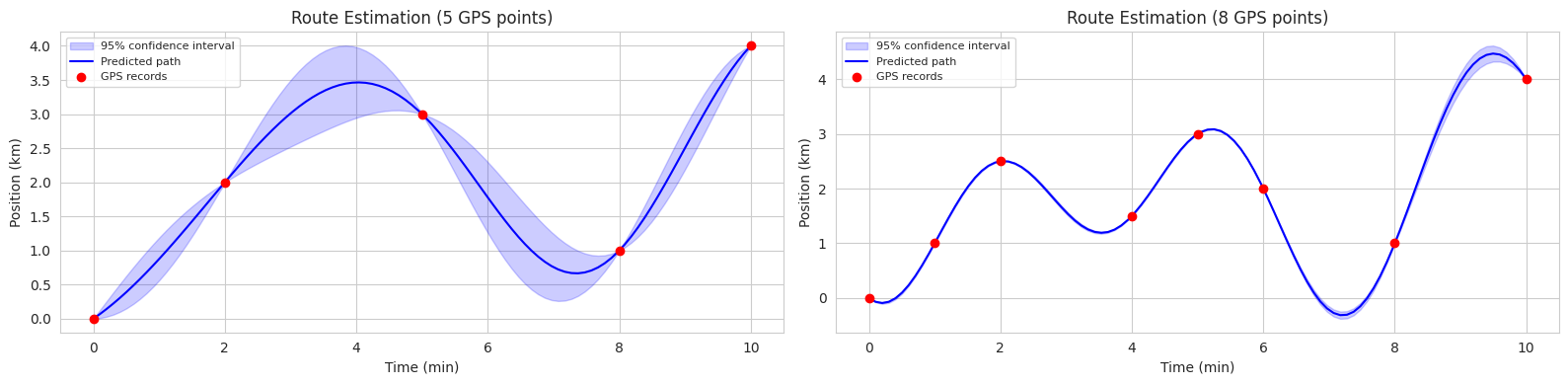
The code above is an example of using GP to estimate bicycle routes in two scenarios (5 observation points, 8 observation points). In each graph, the blue solid line represents the predicted average route, and the blue shaded area represents the 95% confidence interval.
Thus, GP provides not only predictive results but also uncertainty, making it useful in various fields where uncertainty needs to be considered in decision-making processes (e.g., autonomous driving, robot control, medical diagnosis).
Gaussian processes are applied in various scientific and engineering fields such as robot control, sensor network optimization, molecular structure prediction, climate modeling, and astrophysical data analysis. A representative application in machine learning is hyperparameter optimization, which we have already discussed. Another field that requires predictive uncertainty is autonomous driving. By predicting the future position of surrounding vehicles and driving more defensively in areas with high uncertainty, autonomous vehicles can improve safety. Additionally, Gaussian processes are widely used in medical fields to predict patient status changes and in asset markets to predict stock prices and manage risks based on uncertainty. Recently, GP applications have been actively researched in combination with reinforcement learning, generative models, causal inference, and meta-learning.
The most important aspect of Gaussian processes is the kernel (covariance function). Deep learning has strengths in learning representations from data. Combining the predictive power of GP and the representation learning ability of deep learning is a natural research direction. One representative method is deep kernel learning (DKL), which uses neural networks to directly learn kernels from data instead of predefining them like RBF kernels.
The general structure of DKL is as follows:
DKL is being applied in various fields. * Image Classification: Uses CNN to extract image features and GP to perform classification. * Graph Classification: Uses Graph Neural Network (GNN) to extract features from graph structures and GP to perform graph classification. * Molecular Property Prediction: Takes molecular graphs as input and predicts molecular properties (e.g., solubility, toxicity). * Time Series Forecasting: Uses RNN to extract features from time series data and GP to predict future values. Here, we will run a simple example of DKL and examine more detailed content and application cases in Part 2.
Deep Kernel Network
First, we define the deep kernel network. The kernel network is a neural network that learns kernel functions. This neural network takes input data and outputs feature representations. These feature representations are used to calculate the kernel matrix.
import torch
import torch.nn as nn
import torch.optim as optim
from torch.distributions import Normal
import numpy as np
import matplotlib.pyplot as plt
import seaborn as sns

# Set seed for reproducibility
torch.manual_seed(42)
np.random.seed(42)

# Define a neural network to learn the kernel
class DeepKernel(nn.Module):
    def __init__(self, input_dim, hidden_dim, output_dim):
        super(DeepKernel, self).__init__()
        self.fc1 = nn.Linear(input_dim, hidden_dim)
        self.fc2 = nn.Linear(hidden_dim, hidden_dim)
        self.fc3 = nn.Linear(hidden_dim, output_dim)
        self.activation = nn.ReLU()

    def forward(self, x):
        x = self.activation(self.fc1(x))
        x = self.activation(self.fc2(x))
        x = self.fc3(x)  # No activation on the final layer
        return x
The input to a deep kernel network is typically a 2D tensor, where the first dimension is the batch size and the second dimension is the dimension of the input data. The output is a 2D tensor of shape (batch size, feature dimension).
GP Layer Definition
The GP layer takes the output of the deep kernel network and computes the kernel matrix, then calculates the predictive distribution.
import torch
import torch.nn as nn

# Define the Gaussian Process layer
class GaussianProcessLayer(nn.Module):
    def __init__(self, num_dim, num_data):
        super(GaussianProcessLayer, self).__init__()
        self.num_dim = num_dim
        self.num_data = num_data
        self.lengthscale = nn.Parameter(torch.ones(num_dim))  # Length-scale for each dimension
        self.noise_var = nn.Parameter(torch.ones(1))  # Noise variance
        self.outputscale = nn.Parameter(torch.ones(1))  # Output scale

    def forward(self, x, y):
        # Calculate the kernel matrix (using RBF kernel)
        dist_matrix = torch.cdist(x, x)  # Pairwise distances between inputs
        kernel_matrix = self.outputscale * torch.exp(-0.5 * dist_matrix**2 / self.lengthscale**2)
        kernel_matrix += self.noise_var * torch.eye(self.num_data)

        # Calculate the predictive distribution (using Cholesky decomposition)
        L = torch.linalg.cholesky(kernel_matrix)
        alpha = torch.cholesky_solve(y.unsqueeze(-1), L)  # Add unsqueeze for correct shape
        predictive_mean = torch.matmul(kernel_matrix, alpha).squeeze(-1) # Remove extra dimension
        v = torch.linalg.solve_triangular(L, kernel_matrix, upper=False)
        predictive_var = kernel_matrix - torch.matmul(v.T, v)


        return predictive_mean, predictive_var

        return predictive_mean, predictive_var
The input to the GP layer is a 2D tensor of shape (batch size, feature dimension). The output is a tuple containing the predicted mean and variance. The RBF kernel is used for computing the kernel matrix, and Cholesky decomposition is utilized for calculating the predictive distribution to improve computational efficiency. y.unsqueeze(-1) and .squeeze(-1) are used to match the dimensions between y and the kernel matrix.
# 데이터를 생성
x = np.linspace(-10, 10, 100)
y = np.sin(x) + 0.1 * np.random.randn(100)

# 데이터를 텐서로 변환
x_tensor = torch.tensor(x, dtype=torch.float32).unsqueeze(-1)  # (100,) -> (100, 1)
y_tensor = torch.tensor(y, dtype=torch.float32)  # (100,)


# 딥 커널과 GP 레이어를 초기화
deep_kernel = DeepKernel(input_dim=1, hidden_dim=50, output_dim=1)  # output_dim=1로 수정
gp_layer = GaussianProcessLayer(num_dim=1, num_data=len(x))

# 손실 함수와 최적화기를 정의
loss_fn = nn.MSELoss()  # Use MSE loss
optimizer = optim.Adam(list(deep_kernel.parameters()) + list(gp_layer.parameters()), lr=0.01)

num_epochs = 100
# 모델을 학습
for epoch in range(num_epochs):
    optimizer.zero_grad()
    kernel_output = deep_kernel(x_tensor)
    predictive_mean, _ = gp_layer(kernel_output, y_tensor) # predictive_var는 사용 안함
    loss = loss_fn(predictive_mean, y_tensor)  # Use predictive_mean here
    loss.backward()
    optimizer.step()
    if(epoch % 10 == 0):
        print(f'Epoch {epoch+1}, Loss: {loss.item()}')

# 예측을 수행
with torch.no_grad():
    kernel_output = deep_kernel(x_tensor)
    predictive_mean, predictive_var = gp_layer(kernel_output, y_tensor)

# 결과를 시각화
sns.set()
plt.figure(figsize=(10, 6))
plt.plot(x, y, 'bo', label='Training Data')
plt.plot(x, predictive_mean.numpy(), 'r-', label='Predictive Mean')
plt.fill_between(x, predictive_mean.numpy() - 1.96 * np.sqrt(predictive_var.numpy().diagonal()),
                 predictive_mean.numpy() + 1.96 * np.sqrt(predictive_var.numpy().diagonal()),
                 alpha=0.2, label='95% CI')
plt.legend()
plt.show()
Epoch 1, Loss: 4.3467857893837725e-13
Epoch 11, Loss: 3.1288711313699757e-13
Epoch 21, Loss: 3.9212150236903054e-13
Epoch 31, Loss: 4.184870765894244e-13
Epoch 41, Loss: 2.9785689973499396e-13
Epoch 51, Loss: 3.8607078688482344e-13
Epoch 61, Loss: 3.9107123572454383e-13
Epoch 71, Loss: 2.359286811054462e-13
Epoch 81, Loss: 3.4729958167147024e-13
Epoch 91, Loss: 2.7600995490886793e-13/tmp/ipykernel_1408185/2425174321.py:40: RuntimeWarning: invalid value encountered in sqrt
plt.fill_between(x, predictive_mean.numpy() - 1.96 * np.sqrt(predictive_var.numpy().diagonal()),
/tmp/ipykernel_1408185/2425174321.py:41: RuntimeWarning: invalid value encountered in sqrt
predictive_mean.numpy() + 1.96 * np.sqrt(predictive_var.numpy().diagonal()),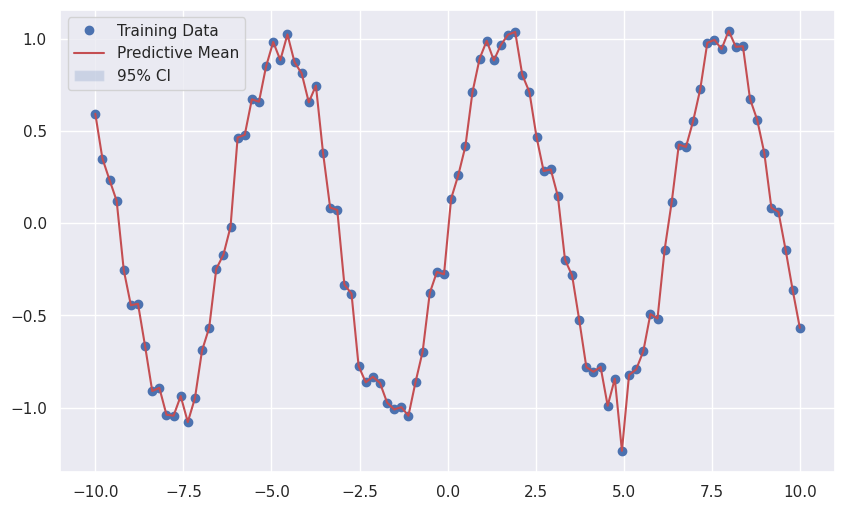
For model learning, the Mean Squared Error (MSE) loss function is used, and the Adam optimizer is used to learn the parameters of the deep kernel network and the GP layer simultaneously.
The previous example shows the basic idea of Deep Kernel Learning (DKL). It uses a deep learning model (the DeepKernel class) to extract features from the input data and calculates the Gaussian Process (GP) kernel using these features. Then, it uses GP to calculate the mean and variance (uncertainty) of predictions. In this way, DKL combines the representation learning ability of deep learning and the uncertainty estimation ability of GP, making reliable predictions possible even for complex data.
Possibilities of DKL:
Limitations of DKL:
This chapter has explored various techniques for addressing the overfitting problem in deep learning models. From traditional methods such as L1/L2 regularization, dropout, and batch normalization, to advanced techniques like Bayesian optimization, Gaussian processes, and Deep Kernel Learning, deep learning research continues to evolve to improve the generalization performance of models.
Overfitting occurs when a deep learning model becomes too specialized to the training data, resulting in poor predictive performance on new data. This can happen when the model’s complexity is too high, when there is insufficient training data, or when the data contains a lot of noise. Preventing overfitting is a crucial task when applying deep learning models to real-world problems.
The various techniques introduced in this chapter approach the overfitting problem in different ways:
custom_loss Lambda Change:
lambda: Increases the influence of the regularization term. Weights become smaller, and the model becomes simpler, increasing the risk of underfitting.lambda: Decreases the influence of the regularization term. Weights become larger, and the model becomes more complex, increasing the risk of overfitting.Polynomial Regression: (Code omitted) If the degree is too high, it overfits; if it’s too low, it underfits.
L1/L2 Regularization: (Code omitted) The stronger the regularization strength (lambda), the smaller the weights become, and performance changes are observed.
Dropout Ratio: (Code omitted) An appropriate dropout ratio can prevent overfitting and improve performance. Too high a ratio can cause underfitting.
Batch Normalization: (Code omitted) Adding batch normalization tends to speed up learning and stabilize convergence.
Lagrange Multiplier Method:
Batch Normalization Backpropagation: (derivation omitted) Batch normalization normalizes the input to each layer, mitigating the vanishing/exploding gradient problem and stabilizing learning.
Loss Plane Visualization: (code omitted) L1 regularization creates a diamond-shaped constraint, while L2 regularization creates a circular constraint, resulting in different optimal solutions.
Dropout Ensemble: Dropout has the effect of training a different network structure each time, similar to ensemble learning. During prediction, all neurons are used (without dropout) to perform an average prediction. Monte Carlo dropout can be used to estimate the uncertainty of predictions.
Hyperparameter Optimization Techniques:
Bayesian Optimization Implementation: (code omitted) Use a surrogate model (e.g., Gaussian process) and an acquisition function (e.g., Expected Improvement) to implement.
Gaussian Process: A probability distribution over functions. Define the covariance between function values using a kernel function. Calculate the posterior distribution based on given data to provide the mean and variance (uncertainty) of predictions.
Kernel Function Conditions: Must satisfy positive semi-definiteness. The kernel matrix (Gram matrix) generated for arbitrary input points must be a positive semi-definite matrix. The RBF kernel satisfies this condition. (proof omitted)
Acquisition Function: Used to determine the next search point in Bayesian optimization. Expected Improvement (EI) considers the possibility of obtaining better results than the current optimal value and the degree of improvement, selecting the next search point accordingly. (equation derivation omitted)
There is no original text to translate.